Headless mode

This example demonstrates how to use the headless mode of chemiscope to generate screenshots programmatically, without running a Jupyter notebook.

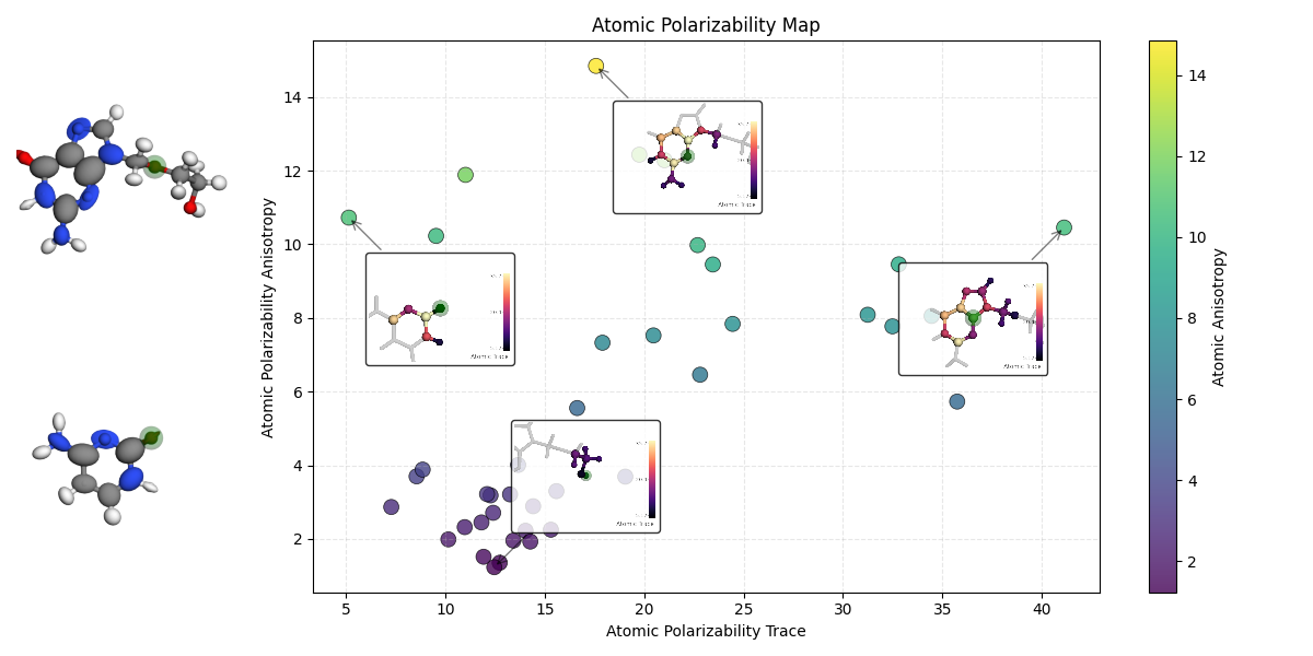
We load a dataset of atomic polarizabilities, visualize it, and then use the headless mode to generate a curated matplotlib plot. We will show snapshots of the two structures in the dataset (with ellipsoids representing polarizability) and detailed views of specific atomic environments (colored by the polarizability trace) embedded in the plot.

import io
import time

import ase.io
import matplotlib.pyplot as plt
import numpy as np
from matplotlib.offsetbox import AnnotationBbox, OffsetImage

import chemiscope
from chemiscope import headless

Load the dataset

We use the alpha-mu dataset which contains atomic polarizability tensors.

structures = ase.io.read("data/alpha-mu.xyz", ":")

Data Processing

We compute the atomic polarizability trace and anisotropy for each atom.

atomic_trace = []
atomic_anisotropy = []

for structure in structures:
    # Construct atomic tensors (Voigt notation: xx, yy, zz, xy, xz, yz)
    # from the individual arrays in the file
    structure.arrays["alpha"] = np.array(
        [
            [axx, ayy, azz, axy, axz, ayz]
            for (axx, ayy, azz, axy, axz, ayz) in zip(
                structure.arrays["axx"],
                structure.arrays["ayy"],
                structure.arrays["azz"],
                structure.arrays["axy"],
                structure.arrays["axz"],
                structure.arrays["ayz"],
                strict=True,
            )
        ]
    )

    alphas = structure.arrays["alpha"]
    for i in range(len(structure)):
        # Voigt to 3x3 matrix
        val = alphas[i]
        tensor = np.array(
            [
                [val[0], val[3], val[4]],
                [val[3], val[1], val[5]],
                [val[4], val[5], val[2]],
            ]
        )

        evals = np.linalg.eigvalsh(tensor)
        trace = np.sum(evals)
        anisotropy = np.abs(evals[2] - evals[0])

        atomic_trace.append(trace)
        atomic_anisotropy.append(anisotropy)

properties = {
    "Atomic Trace": atomic_trace,
    "Atomic Anisotropy": atomic_anisotropy,
}

# Generate environments for all atoms
environments = chemiscope.all_atomic_environments(structures, cutoff=3.5)

Visualization Setup

We define shapes for atomic ellipsoids and settings for the map.

shapes = {
    "alpha": chemiscope.ase_tensors_to_ellipsoids(
        structures, "alpha", force_positive=True, scale=0.2
    )
}

settings = {
    "map": {
        "x": {"property": "Atomic Trace"},
        "y": {"property": "Atomic Anisotropy"},
        "color": {"property": "Atomic Anisotropy"},
    },
    "structure": [
        {
            "shape": "alpha",
            "axes": "off",
            "environments": {
                "activated": False,
                "center": False,
            },
        }
    ],
}

Interactive Widget

In a Jupyter notebook, you would display the widget like this:

cs = chemiscope.show(
    structures,
    properties=properties,
    shapes=shapes,
    settings=settings,
    environments=environments,
)
cs

×

×

To save a screenshot in a notebook, you can use the widget’s save_structure_image method. However, this requires a running notebook kernel and frontend.

cs.save_structure_image("structure.png")

Headless Visualization

We initialize the headless widget. We will use it to capture different types of snapshots.

print("Initializing headless chemiscope...")
headless_widget = headless(
    structures=structures,
    properties=properties,
    shapes=shapes,
    settings=settings,
    environments=environments,
    width=400,  # smaller width for smaller file size
)

# 1. Capture snapshots of the two whole structures with ellipsoids
print("Capturing structure snapshots...")

# Configure for structure view (ellipsoids enabled)
headless_widget.settings = {
    "target": "structure",
    "structure": [
        {
            "shape": "alpha",  # Enable ellipsoids
            "axes": "off",
            "keepOrientation": True,
            "atoms": True,
            "bonds": True,
            # Disable environment highlighting and centering for full structure view
            "environments": {"activated": False, "center": False},
        }
    ],
}

structure_images = []
for i in range(len(structures)):
    # Select the structure (clearing atom selection)
    headless_widget.selected_ids = {"structure": i}
    time.sleep(0.5)  # Wait for render

    img_data = headless_widget.get_structure_image()
    structure_images.append(plt.imread(io.BytesIO(img_data)))


# 2. Capture snapshots of specific atomic environments
print("Capturing atom snapshots...")

# Configure for atom view (color by Trace, no ellipsoids)
headless_widget.settings = {
    "target": "atom",
    "structure": [
        {
            "shape": "",  # Disable ellipsoids
            "color": {
                "property": "Atomic Trace",
                "palette": "magma",
            },  # Use magma palette
            "axes": "off",
            "keepOrientation": False,  # Re-orient for each atom
            "environments": {
                "activated": True,
                "center": True,  # Center on the environment
                "cutoff": 3.5,
                "bgStyle": "licorice",
                "bgColor": "grey",
            },
        }
    ],
}

# Select atoms with min/max Trace and Anisotropy, and some intermediate points
sorted_trace_indices = np.argsort(atomic_trace)
indices_to_show = [
    np.argmin(atomic_trace),
    np.argmax(atomic_trace),
    np.argmin(atomic_anisotropy),
    np.argmax(atomic_anisotropy),
]
indices_to_show = sorted(list(set(indices_to_show)))

atom_images = []
for i in indices_to_show:
    env = environments[i]  # tuple: (structure_index, atom_index, cutoff)
    headless_widget.selected_ids = {"structure": int(env[0]), "atom": int(env[1])}
    time.sleep(0.5)

    img_data = headless_widget.get_structure_image()
    atom_images.append(plt.imread(io.BytesIO(img_data)))

headless_widget.close()

Initializing headless chemiscope...
Capturing structure snapshots...
Capturing atom snapshots...

Generating the Plot

We combine a scatter plot of properties with the captured images.

print("Generating summary plot...")
fig = plt.figure(figsize=(12, 6))
gs = fig.add_gridspec(2, 3, width_ratios=[1, 2, 2])

# Structure 0 (Top Left)
ax_struct0 = fig.add_subplot(gs[0, 0])
ax_struct0.imshow(structure_images[0])
ax_struct0.axis("off")

# Structure 1 (Bottom Left)
ax_struct1 = fig.add_subplot(gs[1, 0])
ax_struct1.imshow(structure_images[1])
ax_struct1.axis("off")

# Main Scatter Plot (Right 2/3)
ax_main = fig.add_subplot(gs[:, 1:])
sc = ax_main.scatter(
    atomic_trace,
    atomic_anisotropy,
    c=atomic_anisotropy,
    cmap="viridis",
    alpha=0.8,
    edgecolors="k",
    linewidths=0.5,
    s=100,
)
cb = plt.colorbar(sc, ax=ax_main, label="Atomic Anisotropy")
ax_main.set_xlabel("Atomic Polarizability Trace")
ax_main.set_ylabel("Atomic Polarizability Anisotropy")
ax_main.set_title("Atomic Polarizability Map")
ax_main.grid(True, linestyle="--", alpha=0.3)

# Add atom snapshots as annotations
for i, img in zip(indices_to_show, atom_images, strict=True):
    # Create image box
    imagebox = OffsetImage(img, zoom=0.12)  # Smaller

    x, y = atomic_trace[i], atomic_anisotropy[i]

    # Determine offset direction to avoid going out of bounds
    x_mean = np.mean(atomic_trace)
    y_mean = np.mean(atomic_anisotropy)

    xybox_x = -60 if x > x_mean else 60
    xybox_y = -60 if y > y_mean else 60

    ab = AnnotationBbox(
        imagebox,
        (x, y),
        xybox=(xybox_x, xybox_y),
        boxcoords="offset points",
        arrowprops=dict(arrowstyle="->", color="black", alpha=0.5),
        bboxprops=dict(facecolor="white", alpha=0.8, boxstyle="round,pad=0.2"),
        frameon=True,
        pad=0.0,
    )
    ax_main.add_artist(ab)

plt.tight_layout()
plt.savefig("headless_curated_plot.png", dpi=150)
print("Plot saved to headless_curated_plot.png")

Generating summary plot...
Plot saved to headless_curated_plot.png